Powder Diffraction

This document provides a comprehensive overview of powder diffraction, a critical analytical technique widely used in materials science, chemistry, geology, and related fields. The International Centre for Diffraction Data (ICDD) supports the advancement of powder diffraction through the development of the Powder Diffraction File (PDF) (Kabekkodu, 2024) and related resources. This article has been adapted from a Wikipedia reference to serve as a standalone resource for the ICDD community.

Introduction

Powder Diffraction is a scientific technique that uses X-rays (commonly abbreviated as PXRD), neutrons (NPD), or electrons to study and characterize solid materials. (Cullity, 1978) It is one of the first and the most used experimental techniques of X-ray crystallography. A common instrument dedicated to performing such measurements is called a powder diffractometer. Powder diffraction measurements can also be performed with cameras equipped with film or by using a goniometer with a variety of detectors. The specimen in a powder diffraction experiment is typically a finely ground powder, the use of which eliminates many specimen-related and instrumental aberrations; however, the powder diffraction method doesn’t require a powder, it can be performed on any polycrystalline sample and is commonly applied to bulk specimens, such as electronic components, artistic pieces, polymer films or other solids.

Powder diffraction is used in a wide variety of diverse applications to measure fundamental material and structural properties, many of which are described in this article. However, the most common application of powder diffraction is to identify and often quantify the components that make up multiphase mixtures. While we will discuss the crystallography and physics of a diffraction pattern, it should be noted that the pattern itself is characteristic of a crystalline solid and can be used to identify materials by comparison to a database of materials. This is much like how fingerprints can be used to identify a person, and therefore, the phase identification portion of the data analysis process is frequently referred to as a “fingerprint” technique for this reason.

Powder X-ray diffraction provides highly consistent results when both sample preparation and instrument calibration are well controlled. Uniform particle size, proper packing, and minimizing preferred orientation are critical for consistent results. Regular calibration using certified standards and instrument health checks are required to ensure the instrument is providing reproducible peak positions and intensities. (JCPDS, 1987)

A few examples of where the technique is being used are listed below.

• Batteries can be evaluated while in use via powder diffraction to evaluate the components of the cell (i.e. cathode, anode, and electrolyte) and how they interact with each other and change structure during operation.
• The composition of soil and rock specimens can be determined and utilized to understand ground stability (Figure 1). A miniaturized diffractometer is on the Mars Rover Opportunity studying the geochemistry of Mars.
• On-site and laboratory diffractometers are used to study the composition of cultural heritage objects to restore and preserve historical artifacts.
• In law enforcement, powder diffraction is used to analyze evidence, determine the authenticity of formulated drugs, and authenticate explosives and explosive residues in forensic analyses.

Figure 1. X-ray powder diffraction from a drill core specimen taken near the San Andreas fault. The experimental data are shown in red at the top. The subsequent data are reference data sets of the minerals identified in the drill core specimen; quartz, albite, laumontite, clinochlore, richterite, microcline, and montmorillonite. Geologists use such data to study ground stability around the fault line.

One of the hallmarks of the powder diffraction method is its versatility. Powder diffraction is useful in nearly every field of human endeavor that requires the characterization and design of materials, which is why the method is widely used by industry, academia, and governments worldwide. The technique is typically performed in the laboratory using X-rays as a radiation source, but it can also be performed with electrons and variable energy X-rays, and neutrons at some of the world’s largest accelerators, synchrotrons, reactors, and spallation sources. The instrumentation can be miniaturized to perform micro-diffraction with specialized focusing optics and/or adopted as microscope attachments using electron diffraction, as shown in Figure 2a. The interpretation of powder diffraction data is facilitated by coherent diffraction from highly crystalline materials, but it can also apply to characteristic incoherent diffraction from semi-crystalline, nano-crystalline, amorphous, and low-dimensional materials (i.e., clays). Powder diffraction is a complementary technique to single crystal diffraction.

Figure 2. (a) A selected area electron diffraction (SAED) pattern, (b) a two-dimensional (2D) X-ray diffraction pattern, (c) an electron back scattered diffraction pattern (EBSD), and (d) a strip detector pattern for powdered aluminum calculated using Cu K-alpha1 (1.54056 Å) radiation and PDF 04-012-7848 in the PDF-5+ 2025 software from the International Centre for Diffraction Data. The inset of 2(b) shows information for the ring that is highlighted in yellow. Aluminum is a face centered cubic (fcc) material of space group Fm-3m.

Explanation

A diffractometer produces electromagnetic radiation (waves) with known wavelength and frequency, which is determined by the type of source that is utilized. The source is often X-rays, because X-ray sources are relatively economical, easy to produce, and readily available. Additionally, the wavelength of X-ray sources, and therefore the corresponding energy, are optimal for interatomic-scale diffraction. However, electrons and neutrons are also common sources, with their frequency determined by their de Broglie wavelength (Kirilyuk, 1999). When these waves reach the sample, the incoming beam is either reflected off the surface or transmitted through the material.  In both cases, a portion of the beam can be diffracted by the atoms which are arranged in a manner that determines the structure (or lack of structure if the material is amorphous) of the material. If the atoms show long-range order, i.e., if the material is crystalline, the ordered atoms at characteristic distances (d) known as d-values or interplanar spacings disperse the incoming X-rays according to Bragg’s Law. (Figure 3)

A geometrical interpretation of diffraction as a reflection process taking place in planes of atoms within a crystal is commonly used to explain the phenomenon, but this simplified explanation does not fully explain the physical process of diffraction.  For simplicity, we will use this geometrical interpretation here. The dispersed X-ray waves will interfere constructively when the path-length difference (2dsinθ) is equal to an integer multiple of the wavelength, producing a diffraction maximum in accordance with Bragg’s law.  At points between the intersection where the waves are out of phase, destructive interference occurs, producing a background signal. Bragg’s law, where λ is the incident wavelength, d is the interplanar spacing, θ is the angle of diffraction, and n is an integer where waves constructively interfere. Both the wavelength and interplanar distances are measured in angstroms (1Å = 0.1 nm = 1 x10^-10 m).

Braggs Law

Figure 3. A schematic diagram of an incident X-ray beam interacting with atoms in a crystalline sample. When the path length difference 2dsinƟ equals an integer multiple of the wavelength, constructive interference occurs, and a peak maximum is noted in the diffraction pattern.

Figure 4.1 illustrates the differences between data collected on (a) single crystals, (b), poorly prepared powder, and (c) ideally prepared powder samples. Single-crystal diffraction works best with a single, macroscopic, well-ordered crystal; whereas powder diffraction works best with randomly oriented crystals that can also be multiphase. The distinction between powder and single crystal diffraction is the degree of in the sample. Single crystals have maximal texturing and are said to be anisotropic. In contrast, in powder diffraction, every possible crystalline orientation is represented equally in an ideal powdered sample, the isotropic case.  In other words, powder X-ray diffraction operates under the assumption that the sample is randomly arranged. Therefore, a statistically significant number of each orientation of the crystal structure will be in the proper orientation to diffract the X-rays. Therefore, all crystallographic d-spacings will be represented in the signal as shown in Figure 4c.  To achieve a statistically significant number of each family of planes, samples are usually ground to a fine particle size, optimally 1-10 microns. In practice, this is often difficult to achieve, and samples are often rotated to improve randomness, which is also called orientation. Figure used with permission from Bob He.

Figure 4.1 is a comparison of (a) single crystal, (b) poorly prepared powder, and (c) ideally prepared powder diffraction patterns. This figure is used with permission from Bob He, a major contributor to the evolution of 2D detector technology, modern diffractometer design, and author of Two-Dimensional X-ray Diffraction. (He, B.B. 2018)

Figure 4.2 This video demonstrates the in-situ recrystallization of a zirconium alloy. Click the play button in the bottom left corner to view the transition of the alloy from α-zirconium powder through the melting process and recrystallization as β-zirconium. The alloy starts as a random powder; the crystallites grow and then melt into a random β powder. With further heating, the random powder agglomerates and orients as the crystal grows. The insert shows the reference patterns for α and β zirconium.

Mathematically, crystals can be described by a 3D ordered arrangement of atoms with some regularity in interatomic distances. Because of this regularity, we can describe this structure in a different way using the reciprocal lattice, which is related to the original structure by a Fourier transform. This three-dimensional space can be described with reciprocal axes  x*, y*, and z* or alternatively in spherical coordinates q, φ*, and χ*. In powder diffraction, intensity is homogeneous over φ* and χ*, and only q remains an important measurable quantity. This is because orientational averaging causes the three-dimensional reciprocal space that is studied in single crystal diffraction to be averaged to the same distribution in all directions of reciprocal space (therefore, it behaves as if it is projected onto a single dimension).

When the scattered radiation is collected on a flat plate detector, as shown in Figure 5, the rotational averaging leads to smooth diffraction rings around the beam axis (Debye-Scherrer rings), rather than the discrete Laue spots (Encyclopedia Britannica, 2025) observed in single crystal diffraction. The angle between the beam axis and the ring is called the scattering angle and in X-ray crystallography, is always denoted as 2θ (in scattering of visible light; the convention is usually θ).

Figure 5: (a) Powder X-ray diffraction experimental setup using a two-dimensional (2D) detector in transmission geometry. (b) 2D powder X-ray diffraction pattern of lanthanum hexaboride standard reference material (LaB6 NIST 660b) obtained at ESRF-ID31 beamline using X-rays of E=75.05 keV (l=0.1652 Å) and (c) the integrated and background-subtracted one-dimensional conventional representation of a PXRD dataset. Parts (b) and (c) are courtesy of Momentum Transfer GmbH . LaB6 is a simple cubic material of space group symmetry type Pm-3m (ICDD PDF 00-034-0427).

This leads to the definition of the scattering vector as:

In this equation, G is the reciprocal lattice vector, q is the length of the reciprocal lattice vector, k is the momentum transfer vector, θ is half of the scattering angle, and λ is the wavelength of the source. Various forms of this equation are found in the literature.

Woolfson, M. M. (1997) instead solves for s as follows:

In this equation, s is the magnitude of the scattering vector (also called the reciprocal lattice vector), d is the interplanar spacing, also called the d-spacing, θ is half of the scattering angle, and λ is the wavelength of the source.

Pecharsky, V. K. (2003) solves for d* as follows: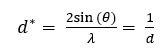

In this equation, d* is the reciprocal lattice spacing, d is the interplanar spacing, also called the d-spacing, θ is half of the scattering angle, and λ is the wavelength of the source.

And Gilmore, C.  (2019) solves for h or s as follows:

In this equation, h is the magnitude of the reciprocal lattice vector, d is the interplanar spacing, also called the d-spacing, θ is half of the scattering angle, and λ is the wavelength of the source.

It follows that:

Powder diffraction data are usually presented as a diffraction pattern (sometimes called a diffractogram) in which the diffracted intensity, I, is shown as a function either of the scattering angle 2θ, d-spacing as determined from θ by Bragg’s Law, or as a function of the scattering vector length q. Both q and d-spacings have the advantage that the diffractogram no longer depends on the value of the wavelength λ. However, the most common expression is the scattering angle 2θ because it is the angle that is recorded by the instrument. Most modern software enables diffraction patterns to be expressed as 2θ, d, or q (x-axis) vs. intensity (y-axis) either as direct counts, square root, log, or log normal counts, depending on user preference. Each type of display has advantages depending on the type of diffraction analysis being conducted.

In practice, a diffraction pattern can be easily explained. The peak locations, as determined by Bragg’s Law, are related to directions where constructive interference occurs among waves diffracted by all the atoms in each crystal; geometrically simplified spacings between planes of atoms within the material. The peak intensity, as shown by Debye and others, is related to the electron density of the crystal and is characteristic of the number, type, and relative position of atoms within the crystal structure. Therefore, each material, having a unique chemical formula and arrangement of atoms, produces a characteristic pattern. In a multiphase pattern, the patterns are additive, and the intensity of each phase is directly related to concentration. Many other applications of powder diffraction, such as the determination of crystallinity, crystallite size, stress, and strain, relate to fundamental changes in the peak profiles.

Uses

Relative to other methods of analysis, powder diffraction allows for rapid, reproducible, non-destructive analysis of multi-component mixtures without the need for extensive sample preparation.[5] This gives laboratories around the world the ability to quickly analyze unknown materials and perform materials characterization in such fields as metallurgy, mineralogy, chemistry, materials science, forensic science, archeology, condensed matter physics, biology, and pharmaceutical sciences. Identification is performed by comparison of the diffraction pattern to a known standard or to a database such as International Centre for Diffraction Data‘s Powder Diffraction File (PDF). Advances in hardware and software, particularly improved optics and fast detectors, have dramatically improved the analytical capability of the technique, especially relative to the speed of the analysis. The fundamental physics upon which the technique is based provides high precision and accuracy in the measurement of interplanar spacings, typically to fractions of an angstrom, resulting in authoritative identification frequently used in patents, criminal cases and other areas of law enforcement. The ability to analyze multiphase materials also allows analysis of how materials interact in a particular matrix such as a pharmaceutical tablet, a circuit board, a mechanical weld, a geologic core sampling, cement and concrete, an electrochemical cell, or a pigment found in a historic painting. The method has been historically used for the identification and classification of minerals, but it can be used for nearly any material, even amorphous ones, if a suitable reference pattern is known, or can be calculated or simulated. The calculation of powder patterns from experimental single crystal structures and their scattering factors enables databases to be calculated from single crystal databases such as the, Inorganic Crystal Structure Database (ICSD), Crystallography Open Database (COD), the Linus Pauling File (Villars, 1998) (LPF), etc. There are also dozens of specialized crystal structure databases that deal with specific fields of science. Experimental reference patterns can contain both coherent and incoherent diffraction contributions, enabling the user to identify amorphous and partially crystalline materials frequently found in polymers, clays, and pharmaceuticals.

Phase identification

The most widespread use of powder diffraction is in the identification and characterization of crystalline solids, each of which produces a distinctive diffraction pattern. Both the positions (corresponding to lattice spacings) and the relative intensity of the lines in a diffraction pattern are indicative of a particular phase and material, providing a “fingerprint” for comparison. A multi-phase mixture, e.g. a soil sample, will show more than one pattern superposed, allowing for the determination of the relative concentrations of phases in the mixture.

J.D. Hanawalt, an analytical chemist who worked for Dow Chemical in the 1930s, realized the analytical potential of creating a database and combining it with a method for unknown identification. Today it is represented by the Powder Diffraction File (PDF) of the International Centre for Diffraction Data (formerly Joint Committee for Powder Diffraction Studies – JCPDS). This has been made searchable by computers through the work of global software developers and equipment manufacturers. There are now over 1.1 million entries in the PDF as of the 2026 release. These databases are interfaced to a wide variety of diffraction analysis software and distributed globally. The Powder Diffraction File contains many subfiles. Examples include minerals, metals and alloys, pharmaceuticals, forensics, excipients, superconductors, semiconductors, etc., with large collections of organic, organometallic and inorganic reference materials.

Crystallinity

In contrast to a crystalline pattern consisting of a series of sharp peaks, amorphous materials (glasses, waxes, etc.) produce a broad background signal. Many polymers show semicrystalline behavior, i.e. part of the material forms an ordered crystallite by folding of the molecule. A single polymer molecule may well be folded into two different, adjacent crystallites and thus form a tie between the two. The tie part is prevented from crystallizing. The result is that crystallinity will never reach 100%. Powder XRD can be used to determine percent crystallinity by comparing the integrated intensity of the background pattern to that of the sharp peaks. Values obtained from powder XRD are typically comparable but not quite identical to those obtained from other methods such as DSC and FTIR. Many, if not most polymers, can be made into an amorphous form by rapid heating and quenching. In fact, there are many techniques used to produce amorphous pharmaceuticals, which are often desirable to obtain high surface areas and increased drug solubility. Powder XRD is frequently used to distinguish crystalline, semi-crystalline, nanocrystalline, and amorphous solids.

Unit cell parameters

The position of a diffraction peak is determined by (1) the atomic positions of the atoms in the unit cell (which relates to the size and shape of the unit cell of a crystalline phase) and (2) the wavelength of the radiation used to collect data if the x-axis is plotted in degrees 2Ɵ.  If the data is plotted with q on the x-axis, the wavelength used is irrelevant.  Each peak represents a certain set of lattice planes and can therefore be characterized by a Miller index. If the symmetry is high, e.g.: cubic or hexagonal, it is usually not too hard to identify the index of each peak, even for an unknown phase. This is particularly important in solid-state chemistry where one is interested in finding and identifying new materials. Once a pattern has been indexed, this characterizes the reaction product and identifies it as a new solid phase. Indexing programs exist to handle the harder cases, but if the unit cell is very large and the symmetry is low (triclinic, monoclinic), success is not always guaranteed.

Expansion tensors, bulk modulus

Unit Cell parameters are temperature and pressure dependent. Powder diffraction can be combined with in situ temperature and pressure control. As these thermodynamic variables are changed, the observed diffraction peaks will migrate continuously to indicate higher or lower lattice spacings as the unit cell distorts. This allows for the measurement of quantities such as the thermal expansion tensor and the isothermal bulk modulus, as well as the determination of the full equation of state of the material. Fundamentally, one can use powder diffraction to analyze the influence of temperature and pressure on any unit cell parameter, as well as any directional vector in the unit cell described by an indexed peak.

Figure 6. This is the thermal expansion of corundum from 120-2200 K. The plot contains the published works of 8 different research groups collected over a period of 55 years (1953-2008). The insert shows the thermal expansion as described by a quadratic equation of the reduced cell volume, over the entire temperature range.

The study of materials as a function of temperature and pressure enables scientists to explore the chemistry of the earth’s core and develop materials useful for the aerospace industry, energy conversion devices, oceanic, and space exploration. It has also led to the development of improved products like better construction materials and cookware.

Phase transitions

At some critical set of conditions, for example at 0 °C for water at 1 atm, a new arrangement of atoms or molecules may become stable when liquid water converts to ice in a physical process known as a phase transition. As commonly taught in most science courses, and defined in the Wikipedia page for phase transitions, “Commonly the term is used to refer to changes among the basic states of matter: solid, liquid, and gas, and in rare cases, plasma.”  Often, however, phase transitions from the perspective of powder diffraction are solid-solid phase transitions; meaning that a transition occurs between different crystalline forms (polymorphs) of the same compound.  When a solid-solid phase transition occurs, new diffraction peaks will appear, and/or old ones disappear according to the symmetry of the new phase in what is called a first order phase transition. If the transition produces another crystalline phase, one set of lines will suddenly be replaced by another set. In some cases, however, lines will split or coalesce, e.g. if the material undergoes a continuous, second-order phase transition. In such cases, the symmetry may change because the existing structure is distorted rather than replaced by a completely different one. For example, the diffraction peaks for the lattice planes (100) and (001) can be found at two different values of d for a tetragonal phase, but if the symmetry becomes cubic, the two peaks will coincide or merge to form one peak.

A famous case of phase transition is the six crystalline forms of chocolate. (Marangoni, A.G., 2011).  The transition and crystallization process at different temperatures is often accompanied by changes in texture, aspect and taste, of obvious interest to chocolate lovers.

Crystal structure refinement and determination

Crystal structure determination from powder diffraction data is extremely challenging due to the overlap of reflections and loss of 3D spatial information when analyzing an isotropic (perfectly randomly oriented crystals) solid. A number of different methods exist for structural determination, derived from the well-developed single-crystal X-ray diffraction technique and specialized for the additional challenges of powder diffraction. The most successful programs, implementing variations of simulated annealing and/or direct methods (crystallography) and related approaches are Fox, DASH, PSSP, EXPO2014, TOPAS , and GSAS-II.

The crystal structures of known materials can be refined (improved in precision and detail from an approximate starting model), i.e. as a function of temperature or pressure, using the Rietveld method. The Rietveld method is a full pattern analysis technique. A model or preliminary crystal structure, together with instrumental and microstructural information, is used to generate a theoretical diffraction pattern for comparison to the observed data. A least squares procedure is then used to minimize the difference between the calculated pattern and each point of the observed pattern by adjusting model parameters. Specialized software for Rietveld refinement can be standalone FULLPROF, BMGN, Maud, Rietan, etc.) or could be found associated with structure determination programs (EXPO2014, TOPAS, and GSAS-II).

Size and strain broadening

There are many factors that determine the width B of a diffraction peak. These include:

• instrumental factors
• the presence of defects to the perfect lattice
• differences in strain in different grains
• the size of the crystallites

In 1918, Paul Scherrer published a paper (Scherrer,1918) which describes the inverse relationship between peak width or breath to crystallite size.  The equation is commonly called the Scherrer equation as follows:

Where B is the breadth of the diffraction peak, k is the Scherrer constant, λ is the wavelength of the radiation, and θ is one-half the diffraction angle. The Scherrer constant depends on the crystallite shape and the size dispersion. The value is typically close to unity.

It is worth noting that the breadth or width of the diffraction peak can be determined in more than one way.  Most commonly, for estimating size via the Scherrer equation, the measure of peak width is reported as the full width at half maximum (FWHM).  It is the distance between two points on the peak profile at half of the maximum intensity.  It is typically reported in degrees of 2θ or in radians.

Alternatively, peak breadth can be expressed as the integral breadth, which is the ratio of the peak area to its maximum height. It represents the width of a rectangle that has the same area and height as the peak.  Integral breadth is often used in line profile analysis because it accounts for the entire peak shape, not just the half-maximum region.

Klug and Alexander (Klug, H. P., & Alexander, L. E., 1974) discuss peak breath in depth and include a correction for instrumental broadening, which is the artificial widening of a diffraction peak caused by the X-ray diffraction instrument rather than the sample itself.  It occurs because every instrument has a finite resolution due to factors like imperfections in the optics, which distort the theoretically ideal sharp peaks.  Analysts use an instrument broadening standard, such as lanthanum hexaboride (LaB₆), to correct the effect of instrument broadening.  The National Institute of Standards and Technology (NIST, 2015) in the United States has traditionally offered this material for purchase.

It is often possible to separate the effects of size and strain. When size broadening is independent of angle (k=1/d), strain broadening increases with increasing angle. In most cases, there will be both size and strain broadening. It is possible to separate these by combining the two equations in what is known as the Williamson–Hall method (Williamson, G.K. & Hall, W.H., 1953):

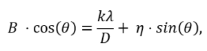
Thus, when we plot B cos⁡(θ)vs. sin⁡(θ), we get a straight line with slope η and intercept kλ/D.

The expression is a combination of the Scherrer equation  (Scherrer,1918) for size broadening and the Stokes and Wilson expression for strain broadening. The value of η represents the strain in the crystallites, and D represents the size of the crystallites.

Frequently, strain and size effects on crystallites are anisotropic, producing peak widths that depend on hkl and on angle (or q). This is particularly important in so-called low-dimensionality materials such as fibrous or lamellar crystal structures. A generalization of the previous equations to include crystal direction-dependent broadening parameters has been derived.

Modern Rietveld software allows one to automatically compute, from the refined profile parameters, both isotropic and anisotropic size and strain parameters, provided that a calibration for the instrumental broadening is given.

Comparison of X-ray and neutron scattering

X-ray photons scatter by interaction with the electron cloud of the material; neutrons are scattered by the nuclei, producing neutron diffraction. This means that, in the presence of heavy atoms with many electrons, it may be difficult to detect light atoms by X-ray diffraction. In contrast, the neutron scattering lengths of nuclei are independent of the atomic number and are approximately equal in magnitude. Neutron diffraction techniques may therefore be used to detect light elements such as oxygen or hydrogen in combination with heavy atoms or distinguish among nearby elements with very similar number of electrons. The neutron diffraction technique therefore has obvious applications to problems such as determining oxygen displacements in materials like high temperature superconductors and ferroelectrics, Li ions in batteries or to hydrogen bonding in biological systems.

As neutrons also have a magnetic moment, they are additionally scattered by any atomic magnetic moments in a sample. In the case of long-range magnetic order, this leads to the appearance of new Bragg reflections or additional intensity in the peaks present. In most cases, neutron powder diffraction may be used to determine the size of the moments and their spatial orientation (so called magnetic structure).

Aperiodically arranged clusters

Predicting the scattered intensity in diffraction patterns from gases, liquids, and randomly distributed nanoclusters in the solid state is (to first order) done rather elegantly with the Debye scattering equation: (Scardi, 2016)

where the magnitude of the scattering vector q is in reciprocal space units (typically Å^-1 or nm^-1), N is the number of atoms, fi(q) is the atomic scattering factor for atom i and scattering vector q, while rij is the distance between atom i and atom j. One can also use this to predict the effect of nano-crystallite shape on detected diffraction peaks, even if in some directions the cluster is only one atom thick.

Semi-quantitative analysis

Semi-quantitative analysis of polycrystalline mixtures can be performed by using traditional methods such as the Relative Intensity Ratio (RIR) or whole-pattern methods using Rietveld Refinement or PONCKS (Partial or No Known Crystal Structures) method. The use of each method depends on the knowledge of the analyzed system, given that, for instance, Rietveld refinement needs the solved crystal structure of each component of the mixture to be performed.

The ability to perform complex multiphase quantitation in the timeframe of single analysis has large implications on industrial throughput and productivity. Rietveld analyses are routinely used by some of the world’s largest materials industries (cement, mining) and are included in most commercial software packages sold with diffraction equipment. In many of these cases, the scale factors and unit cell parameters are being refined.

Quantitative methods are continuously being developed with modifications and improvements to the methods mentioned above, including hybrid techniques which address non-crystalline samples and those that combine complementary analytical data. In the last decades, multivariate analysis has spread as a complementary method for phase quantification.

Traditional analytical methods such as standard calibration and standard addition are also useful with powder XRD. While more intensive, usually requiring multiple samples for each analyte, the results are often more accurate and precise.

Devices

Cameras

The simplest cameras for X-ray powder diffraction consist of a small capillary and either a flat plate detector (originally a piece of X-ray film, now more and more a flat-plate detector or a CCD-camera) or a cylindrical one (originally a piece of film in a cookie-jar, but increasingly bent position sensitive detectors are used). The two most frequently used types of cameras are the Laue and the Debye–Scherrer camera.

To ensure complete powder averaging, the specimens are finely ground, and the capillary is usually spun around its axis.

The Guinier camera is built around a focusing bent crystal monochromator. The sample is usually placed in the focusing beam, e.g., as a dusting on a piece of sticky tape. A cylindrical piece of film (or electronic multichannel detector) is put on the focusing circle, but the incident beam is prevented from reaching the detector to prevent damage from its high intensity. The main advantage of a Guinier camera is the high resolution provided by the focusing optics and crystal monochromator. Cameras based on hybrid photon counting technology, such as the PILATUS detector from Dectris, are widely used in applications where high data acquisition speeds and increased data quality are required.

For neutron diffraction, vanadium cylinders are used as sample holders. Vanadium has a negligible absorption and coherent scattering cross section for neutrons and is hence nearly invisible in a powder diffraction experiment.

Diffractometers

Figure 7. Hemisphere of diffraction showing the incoming and diffracted beams K₀ and K (or S₀ and S, depending on the literature) that are inclined by an angle of θ with respect to the sample surface. This image represents a Ɵ-Ɵ configuration.

Diffractometers can be operated both in transmission and reflection geometry, but reflection is more common in conventional laboratory instruments using Cu Ka radiation. The powder sample is loaded in a small disc-like container, and its surface is carefully flattened. The disc is put on one axis of the diffractometer and tilted by an angle θ while a detector (scintillation counter is one type) rotates around it on an arm at twice this angle. This configuration is known as the Bragg–Brentano θ-2θ configuration.

Another configuration is the Bragg–Brentano θ-θ configuration in which the sample is stationary while the X-ray tube and the detector are rotated around it. The angle formed between the x-ray source and the detector is 2θ. This configuration is most convenient for loose powders and simplifies the use of multiple sample stages on a single diffractometer.

Diffractometer settings for different experiments can schematically be illustrated by a hemisphere, in which the powder sample resides in the origin. The case of recording a pattern in the Bragg-Brentano θ-θ mode is shown in Figure 7, where K0 and K stand for the wave vectors of the incoming and diffracted beam that both make up the scattering plane. Various other settings for texture or stress/strain measurements can also be visualized with this graphical approach.

Position-sensitive detectors (PSD) and area detectors, which allow collection from multiple angles at once, are becoming more popular on currently supplied instrumentation.

Neutron diffraction

Sources that produce a neutron beam of suitable intensity and wavelength for diffraction are only available at a small number of research reactors and spallation sources in the world. Angle dispersive (fixed wavelength) instruments typically have a battery of individual detectors arranged in a cylindrical fashion around the sample holder and can therefore collect scattered intensity simultaneously on a large 2θ range. Time of flight instruments normally had a small range of banks at different scattering angles which collected data at varying resolutions; however, modern instruments are equipped with hundreds of detectors at all angles within and out of the diffraction plane to obtain data at faster rates.  POWGEN, located at Oak Ridge National Laboratory, is an example of a high-resolution neutron powder diffractometer.

Neutron diffraction has never been an in-house technique because it requires the availability of an intense neutron beam which is only available at a nuclear reactor or spallation source. Typically, the available neutron flux and the weak interaction between neutrons and matter require relatively large samples.

X-ray tubes

Laboratory X-ray diffraction equipment relies on the use of an X-ray tube, which is used to produce the X-rays. Copper anode X-ray tubes are most common, but cobalt and molybdenum are also popular. The wavelength in nm varies for each source. The table below shows these wavelengths, determined by Bearden (Bearden, J. A., 1967) and quoted in the International Tables for X-ray Crystallography (all values in nm):

Element	Kα2	Kα1	Kβ
Cr	0.2293663	0.2289760	0.2084920
Co	0.1792900	0.1789010	0.1620830
Cu	0.1544426	0.1540598	0.1392250
Mo	0.0713609	0.0709319	0.0632305

Note that most commercial diffractometer systems, and XRD powder diffraction application software, will cite these values in angstroms. (x10 in the above Table).

Other sources

In-house applications of X-ray diffraction have always been limited to the relatively few wavelengths shown in the table above. The available choice was much needed because the combination of certain wavelengths and certain elements present in a sample can lead to strong fluorescence which increases the background in the diffraction pattern. A notorious example is the presence of iron in a sample when using copper radiation. In general, elements showing absorption edges at energies just below the anode element’s emission energy should be avoided.

Another limitation is that the intensity of traditional generators is relatively low, requiring lengthy exposure times and precluding any time-dependent measurement. The advent of synchrotron sources has drastically changed this picture and caused powder diffraction methods to enter a whole new phase of development. Not only is there a much wider choice of wavelengths available, but the high brilliance of the synchrotron radiation makes it possible to observe time-sensitive changes in the pattern during chemical reactions, temperature ramps, pressure changes, etc. Tremendous advances in detector technology, both in energy resolution and photon efficiency, now enable time-dependent measurements with all types of diffraction equipment. Data collection time scales are typically several minutes for laboratory sources and as little as fractions of a second with a synchrotron.

The tunability of the wavelength also makes it possible to observe anomalous scattering effects when the wavelength is chosen close to the absorption edge of one of the elements of the sample.

Advantages and disadvantages

Powder X-ray diffraction is a powerful and useful technique. It is mostly used to characterize, identify, and quantify phases, frequently in mixtures, but as described above, there are many other applications. Like any analytical technique, the method has both advantages and disadvantages.

Advantages of the technique are:

• the non-destructive nature of the method
• can differentiate between crystalline and amorphous materials
• simplicity of sample preparation (in most cases)
• rapidity of measurement
• the ability to analyze mixed phases, e.g. soil samples
• well suited for “in situ” analyses, that can include structure determination, thermal behavior, on-site forensic analysis, mineralogy, and analysis of objects with cultural heritage
• provides bulk information representative of a statistically significant volume of material
• provides information on how materials interact in mixtures

Disadvantages of the technique are:

• detection limits are relatively high (weight percent)
• sensitive to sample preparation techniques
• relatively high instrumentation cost
• considerable knowledge may be needed to correctly interpret the data

Many materials are readily available with sufficient microcrystallinity for powder diffraction, or samples may be easily ground from larger crystals. In the fields of solid-state chemistry, catalysis, or pharmaceutical chemistry that often aim at synthesizing new materials, single crystals thereof are typically not immediately available.

Since all possible crystal orientations are measured simultaneously, collection times can be quite short even for small and weakly scattering samples. This is not merely convenient but can be essential for samples which are unstable either inherently or under X-ray or neutron bombardment, or for time-resolved studies.

In recent years advances in sources, optics and detectors have improved time-resolved powder diffraction in accuracy, power, and speed, independent of whether the source is a synchrotron, lab, benchtop instrument, or portable instrument such as a Mars rover.

References

B.D. Cullity Elements of X-ray Diffraction Addison Wesley Mass. (1978) ISBN 0-201-01174-3

Bearden, J. A. (1967). “X-Ray Wavelengths”. Reviews of Modern Physics. 39 (1): 78–124. DOI: https://doi.org/10.1103/RevModPhys.39.78

Gilmore, C. J., Kaduk, J. A., & Schenk, H. (Eds.). (2019). International tables for crystallography: Volume H, powder diffraction (Vol. H). Wiley Blackwell.

He, B. B. (2018). Two dimensional X-ray diffraction (2nd ed.). John Wiley & Sons. ISBN 9781119356097.

JCPDS–International Centre for Diffraction Data. (1987). Methods & practices in X-ray powder diffraction. Swarthmore, PA: JCPDS–International Centre for Diffraction Data.

Kabekkodu, S., Dosen, A., and Blanton T. (2024). “PDF-5+: a comprehensive Powder Diffraction File™ for materials characterization.” Powder Diffraction 39(2): 47-59. doi:10.1017/S0885715624000150

Kirilyuk, A. P. (1999). 75 Years of Matter Wave: Louis de Broglie and Renaissance of the Causally Complete Knowledge. arXiv preprint quant-ph/9911107.

Klug, H. P., & Alexander, L. E. (1974). X-ray diffraction procedures: For polycrystalline and amorphous materials (2nd ed.). New York: Wiley-Interscience ISBN: 978-0471493693

Marangoni, A.G. (2011), “Edible nanostructures – the pleasures of chocolate”, plenary speaker Denver X-ray Conference.and Stobbs, J.A., Ghazani, S.M., Donnelly, M-E, and Marangoni, A.G”, (2025), “Chocolate temperating: A perspective” Crystal Growth & Design 25 (9), 2764-2783.

National Institute of Standards and Technology (NIST). (2015). Standard Reference Material 660c: Line Position and Line Shape Standard for Powder Diffraction (Lanthanum Hexaboride Powder). Gaithersburg, MD: NIST. Retrieved from https://tsapps.nist.gov/srmext/certificates/660c.pdf

Pecharsky, V. K., & Zavalij, P. Y. (2003). 1.15 Reciprocal Lattice. In Fundamentals of Powder Diffraction and Structural Characterization of Materials (pp. 50–52). essay, Springer.

Scardi, P., Billinge, S. J. L., Neder, R., & Cervellino, A. (2016). Celebrating 100 years of the Debye scattering equation. Acta Crystallographica Section A: Foundations and Advances, 72(6), 589–590. https://doi.org/10.1107/S2053273316015680

Scherrer, P. (1918). Bestimmung der Grösse und der inneren Struktur von Kolloidteilchen mittels Röntgenstrahlen. Nachrichten von der Gesellschaft der Wissenschaften zu Göttingen, Mathematisch-Physikalische Klasse, 26, 98–100.

The Editors of Encyclopedia Britannica. “Laue diffraction.” Encyclopedia Britannica, 12 Mar. 2025. https://www.britannica.com/science/Laue-diffraction. Accessed 15 Oct. 2025.

Villars, P., Onodera, N., & Iwata, S. (1998). The Linus Pauling file (LPF) and its application to materials design. Journal of Alloys and Compounds, 279, 1–7. https://doi.org/10.1016/S0925-8388(98)00605-7

Wikipedia contributors. (n.d.). Miller index. Wikipedia. Retrieved October 15, 2025, from https://en.wikipedia.org/wiki/Miller_index [en.wikipedia.org]

Wikipedia contributors. (n.d.). Solid-state chemistry. Wikipedia. Retrieved October 15, 2025, from https://en.wikipedia.org/wiki/Solid-state_chemistry

Williamson, G. K., & Hall, W. H. (1953). X-ray line broadening from filed aluminium and wolfram. Acta Metallurgica, 1(1), 22–31. https://doi.org/10.1016/0001-6160(53)90006-6

Woolfson, M. M. (1997). The scattering of X-rays. In An Introduction to X-ray Crystallography (2nd ed., pp. 45–63). Cambridge University Press.